Algorithm
DNA step parameters
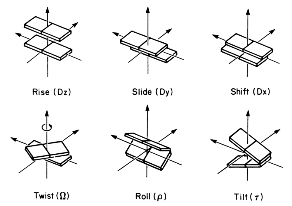
The diagram below shows the six main ways that two consecutive base pairs are distanced from each other.

Of these six, the three parameters SymCurve uses are \(\Omega\), \(\rho\), and \(\tau\). Also, SymCurve uses estimates of the 3-mer version of these parameters instead of the 2-mer representations in the diagram. These parameters \(\Omega\), \(\rho\), and \(\tau\) in this case take the form of 4x4x4 matrices, with one dimension per nucleotide in the 3-mer.
For the roll parameter \(\rho\), SymCurve uses one of two matrices: \(\rho^\alpha\) representing roll in an “active” state, where polymerases may be actively transcribing the DNA, or \(\rho^\beta\) representing roll in a “simple” or “inactive” state.
3-mer windowing
In our equations later, we’ll refer to the input nucleotide sequence as \(S\), with length \(n\). Individual nucleotides \(s_i\) form \(S\) as in the notation below:
\[S = \left(s_1,s_2,...,s_{n-1},s_n\right)\]Then we’ll define \(W\) as the set of all sliding-window 3-mer subsequences \(w_i\) of \(S\) such that:
\[ \begin{aligned} W &= \left(w_1,w_2,...,w_{n-3},w_{n-2}\right) \\ W &= \left[\left(s_1,s_2,s_3\right),\left(s_2,s_3,s_3\right),...,\left(s_{n-3},s_{n-2},s_{n-1}\right),\left(s_{n-2},s_{n-1},s_n\right)\right] \end{aligned} \]As additional shorthand we’ll define the lookup of a given 3-mer \(w_i\) in the \(4\times 4 \times 4\) matrices \(\Omega\), \(\rho\), and \(\tau\) as \(\Omega_i\), \(\rho_i\), and \(\tau_i\) respectively. The matrix values at each window are used to compute variables \(T_i\) (the cumulative twist-sum), and the deltas \(dx_i\) and \(dy_i\), also for each window:
\[ \begin{aligned} T_i &= \sum_{j=1}^{i}\Omega_j \\ dx_i &= \rho_i \sin(T_i) + \tau_i \sin(T_i - \pi/2) \\ dy_i &= \rho_i \cos(T_i) + \tau_i \cos(T_i - \pi/2) \end{aligned} \]Mapping into 2D space
Across the space of \(n-2\) 3-mers \(w_i\), we’ll define \(x_i\) and \(y_i\) coordinates as the sum of the previous coordinates/deltas as:
\[ \begin{aligned} x_{i+1} &= x_i + dx_i \\ y_{i+1} &= y_i + dy_i \end{aligned} \]where \(x_1 = y_1 = 0\). Note: the range of valid coordinates \(i\) extends to \(n-1\), which is one past the number of 3-mer windows. For this reason, \(x_1\) and \(y_1\) are ignored in subsequent steps.
Rolling coordinate averages
We’ll now define a parameter \(a\), where \(2a+1\) is a sliding window size over the range of coordinates \(a+1 \lt i \lt n-a-1\). Usually, we set \(a=5\) which means a sliding window of 11 bases ecompasses the rolling average. The rolling averages \(\overline{x}\) and \(\overline{y}\) are also slightly weighted centrally, with the values at either end of the window only contributing half what the central values contribute.
\[ \begin{aligned} \overline{x}_i &= \left(\frac{x_{i-a-1}+x_{i+a+1}}{2} + \sum_{j=i-a}^{i+a}x_j\right)\left(\frac{1}{2a+2}\right) \\ \overline{y}_i &= \left(\frac{y_{i-a-1}+y_{i+a+1}}{2} + \sum_{j=i-a}^{i+a}y_j\right)\left(\frac{1}{2a+2}\right) \\ \end{aligned} \]Curvature
Using the rolling averages, the curvature values \(\kappa_i\) are now possible to calculate over a range of \(a+b+1 < i < n-a-b-1\) where \(b\), is another half-span, usually set to 15. \(\kappa_i\) is computed as the Euclidean distance between the points \((\overline{x}_{i+b}, \overline{y}_{i+b})\) and \((\overline{x}_{i-b}, \overline{y}_{i-b})\). Additionally, a scaling coefficient \(\lambda\) is applied and by default set to \(0.33335\).
\[ \kappa_i = \lambda\sqrt{(\overline{x}_{i+b}-\overline{x}_{i-b})^2 + (\overline{y}_{i+b}-\overline{y}_{i-b})^2} \]Symmetry
The final step is to calculate the symmetry of the curvature values. A final span parameter \(c\) is usually set to 51 so that the symmetry values \(\xi_i\) can be calculated over the range of \(2c < i < 2c-1\). Actually, if \(2c > a + b + c\), there are missing symmetry values in the output that could potentially be computed. For now, the SymCurve algorithm is meant to match the original implementation as closely as possible.
(more coming soon)